Fisheries management is a process that regulates how much fish commercial, recreational and subsistence fisher folk can harvest. Management strategies can take many forms, but the basic goals of most modern fisheries management are to preserve healthy and self-sustaining fish populations while simultaneously maximizing harvest for the benefit of the fishers.
Note: two important terms in fisheries management are “stock”, which is the term for a population of fish being managed as a single geographic unit (often but not always a single species), and “biomass”, which is the average weight of fish multiplied by the number of fish, and is the typical measurement unit for fish populations, rather than number of individuals.
In order to determine what a healthy and self-sustaining population for a given stock is, fisheries scientists use statistical modeling to project current, past and future stock biomasses. There are many different statistical models that are used, as different areas and species have different contexts, and different knowledge gaps that need to be overcome. Fisheries scientists are continually looking for ways to improve our statistical models to get more accurate and precise estimates of biomass which will then hopefully get us closer and closer to maximizing both management goals of preserving self-sustaining populations and maximizing harvest.
Study Area
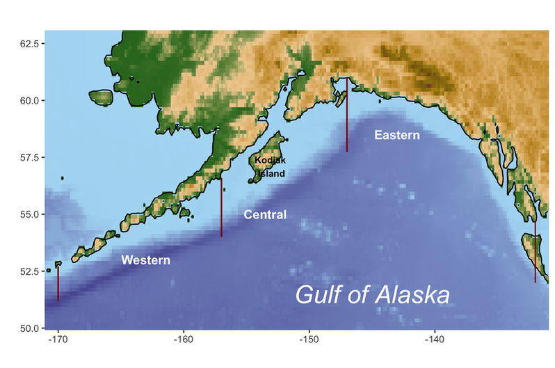
My thesis project work is aimed at improving the model used to estimate stock biomass for several stocks in the Gulf of Alaska commercial groundfish fishery. This particular fishery is an economically important one, both to local Alaskan fishers throughout the Gulf as well as to other US commercial fishers who come up from Seattle or other parts of the West Coast. Groundfish is a management category of several fish species that are generally found on or near the seabed of continental shelves, areas of the ocean that are relatively shallow and occur just offshore of coastlines (shown in light blue in the map below). In the commercial fishery, they are harvested primarily with bottom trawls, nets that are dragged across the seabed. Many groundfish stocks in the Gulf are managed using subregions, meaning that harvest rules are allocated across each of three subregions (western, central and eastern, shown on the map below with red lines delineating their borders) based on the stock’s estimated biomass in that subregion. This approach is used primarily to preserve local populations of stocks by ensuring that areas that are easier to fish or closer to fishing communities aren’t fished too heavily.
Unfortunately, a lot is still unknown about the biology and ecology (their behavior, habitat requirements and role in their ecosystem) of most groundfish species, which makes it more challenging to model their population dynamics. In the Gulf of Alaska, commercial groundfish fishing exploded in the 1960s and 70s, and some stocks subsequently experienced significant decreases in population. Although it is not usually possible to say definitively that a stock’s decline is due directly to overfishing (there may be coinciding environmental variables that are contributing to a decline), once a population is clearly in decline, fisheries managers become concerned that overfishing may occur and drive the stock into even further decline. Consequently, commercial fishing for this fishery was regulated much more strictly starting in the 1980s, and many of the stocks have experienced increases in population since then. Because of this decline and subsequent recovery, these stocks are managed carefully.
Study Species
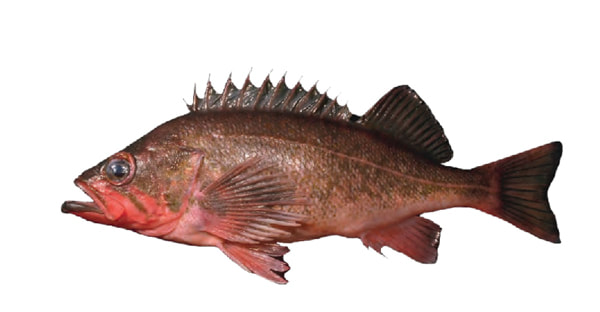
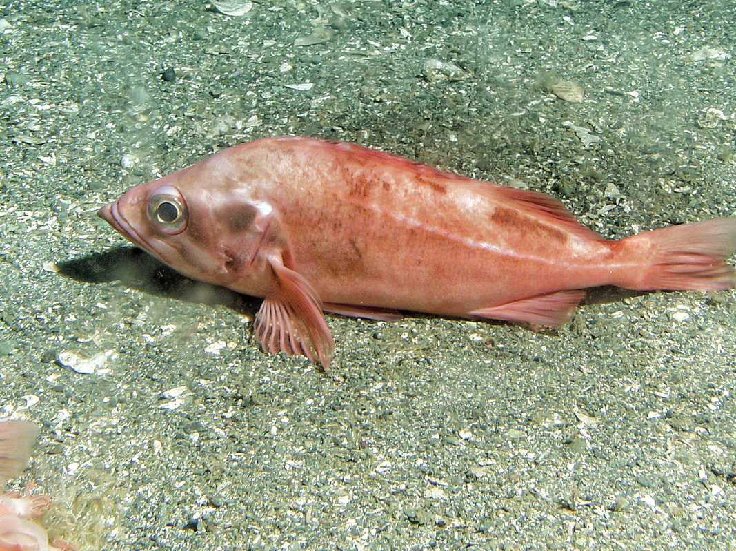
My work focuses on two species that are managed as single species stocks - Pacific Ocean Perch (Sebastes alutus) and Northern Rockfish (Sebastes polyspinis). These are two of the most economically important stocks in this fishery. Pacific Ocean Perch alone accounts for 70% of the catch in the Gulf of Alaska groundfish fishery. In 2019 the catch for Pacific Ocean Perch was worth $23.9 million while Northern Rockfish catch was worth $2.4 million.
Because it is a more valuable species, a bit more is known about Pacific Ocean Perch ecology, such as that they undergo a seasonal migration where they move from deeper parts of the continental shelf (300 - 420 meters) in the winter to shallower parts (150 - 300 m) in the summer. They also don’t spend all of their time at the bottom, but will come up higher in the water column during the day, likely to feed. Both Pacific Ocean Perch and Northern Rockfish are slow maturing and long-lived, like most rockfish species - the oldest Pacific Ocean Perch captured in the Gulf was 84 years old, and the oldest Northern Rockfish was 67. Very little is known about the larval or juvenile stages of either species, and even less is known about Northern Rockfish adults’ behavior than Pacific Ocean Perch, other than the fact that they live up to their name and appear to prefer rocky bottom habitat that is difficult to trawl.
Because it is a more valuable species, a bit more is known about Pacific Ocean Perch ecology, such as that they undergo a seasonal migration where they move from deeper parts of the continental shelf (300 - 420 meters) in the winter to shallower parts (150 - 300 m) in the summer. They also don’t spend all of their time at the bottom, but will come up higher in the water column during the day, likely to feed. Both Pacific Ocean Perch and Northern Rockfish are slow maturing and long-lived, like most rockfish species - the oldest Pacific Ocean Perch captured in the Gulf was 84 years old, and the oldest Northern Rockfish was 67. Very little is known about the larval or juvenile stages of either species, and even less is known about Northern Rockfish adults’ behavior than Pacific Ocean Perch, other than the fact that they live up to their name and appear to prefer rocky bottom habitat that is difficult to trawl.
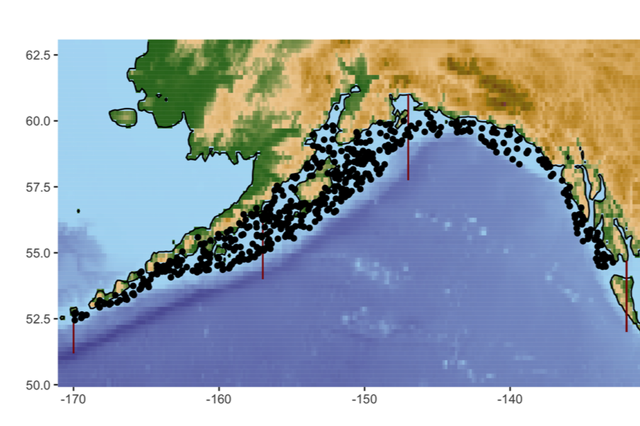
Statistical models require data in order to make estimates, and collecting data at regular intervals using the same methods is an enormous part of the work that fisheries scientists undertake in order to maintain good datasets to use for models. For this groundfish fishery, a bottom trawl survey run by the National Oceanic & Atmospheric Administration (NOAA) has been operating in the Gulf of Alaska every 2 or 3 years since the 1980s. This is a multi-species survey, meaning that they are not trying to catch any particular groundfish species, and it is done using a stratified random sampling spatial method. Stratified random sampling means that the study area is sectioned out in some way (stratified) and within each section random locations are drawn to sample. The stratification criteria used for this survey is depth (with a maximum depth of 1000 m), and a minimum of 2 sample locations for each depth section is randomly selected to be included in the survey for each year. Ensuring random sampling in a survey design is very important because it allows us to assume that the data we produce is a random, unbiased sample of the population and makes it easier to estimate that population based on the sample collected. A significant challenge that this survey encounters is that large amounts of the continental shelf in the Gulf is very rocky, making it difficult or impossible to trawl.
An example of the locations surveyed in one year (2019) is shown in the map below, where each point is the starting latitude and longitude of a single 15 minute trawl period. The data I am using starts in 1990 and ends in 2019 for Pacific Ocean Perch (for a total of 14 years of survey data) and starts in 1984 and ends in 2019 for Northern Rockfish (for a total of 16 years of survey data).
An example of the locations surveyed in one year (2019) is shown in the map below, where each point is the starting latitude and longitude of a single 15 minute trawl period. The data I am using starts in 1990 and ends in 2019 for Pacific Ocean Perch (for a total of 14 years of survey data) and starts in 1984 and ends in 2019 for Northern Rockfish (for a total of 16 years of survey data).
Study objectives
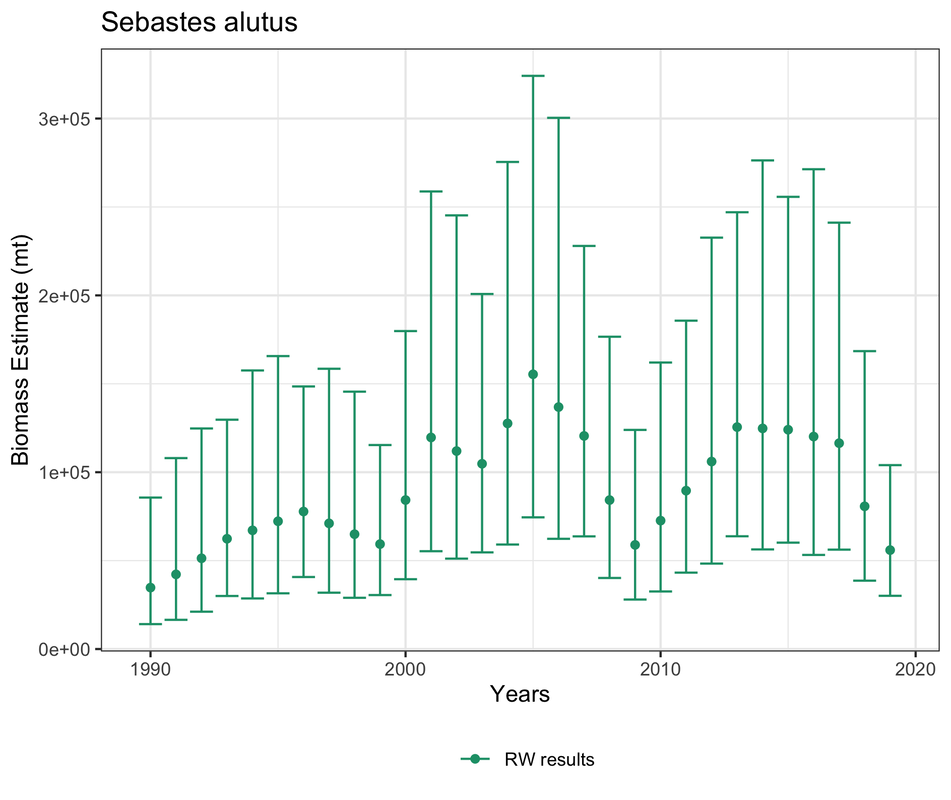
The modeling approach that is currently used to estimate stock biomass for these stocks, called a random walk model, has a high amount of uncertainty, meaning that the predictions are not very precise. The consequence of this is that in order to preserve the management objective to maintain healthy self-sustaining stock populations, management rules have to be fairly conservative and the other management objective is not being met because harvest is likely not being maximized. Below is an example of predicted biomass estimates from the random walk model for Pacific Ocean Perch in the western subregion, with the points representing the estimates and the lines representing 95% confidence intervals. Notice that for some estimates, the confidence intervals have an over 200,000 metric ton range of uncertainty, which is enormous room for error.
In this project, I work with a spatio-temporal model (meaning it uses both time and space as variables), and the primary objective is to improve the precision of estimates compared to the random walk model and ideally match or improve on the random walk model in terms of accuracy of estimates compared to the bottom trawl survey data.
Additionally, because these species are so long lived and slow to mature, it is reasonable to assume that the population wouldn’t change an enormous amount from year to year. Unfortunately, the survey data fluctuates quite a bit from year to year, likely more due to encountering untrawleable habitat, other environmental factors like weather interfering with the trawl route, or human error such as misidentification of captured fish than to true change in biomass. The random walk model is quite sensitive to this fluctuation, and consequently there is a good chance that predictions for one year will be quite different from the year before, making it more difficult for fishers to plan ahead for each fishing season and requiring managers to revisit harvest rules each year. Therefore, a further objective of my study is to hopefully produce estimates with less variability from year to year.
Additionally, because these species are so long lived and slow to mature, it is reasonable to assume that the population wouldn’t change an enormous amount from year to year. Unfortunately, the survey data fluctuates quite a bit from year to year, likely more due to encountering untrawleable habitat, other environmental factors like weather interfering with the trawl route, or human error such as misidentification of captured fish than to true change in biomass. The random walk model is quite sensitive to this fluctuation, and consequently there is a good chance that predictions for one year will be quite different from the year before, making it more difficult for fishers to plan ahead for each fishing season and requiring managers to revisit harvest rules each year. Therefore, a further objective of my study is to hopefully produce estimates with less variability from year to year.
Overview of project steps
|
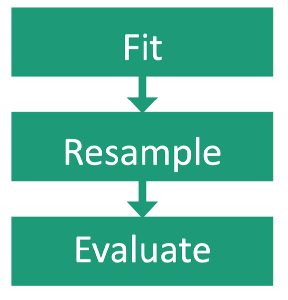
The first step of this project is to fit both the random walk and spatio-temporal model to the survey data. In an ideal world, I would have multiple independent data sets available and I would fit the models to each data set in order to compare how well the models work using a range of inputs. However, in ecology there is very rarely more than one dataset available, and that is unfortunately true in this case. To overcome this obstacle, the survey data is resampled by taking different data points out each time to create multiple slightly different data sets and the models are fit to each of these. Once there are a range of results to work with, I will use several metrics measuring accuracy and precision to evaluate how well the models perform comparatively.
|
Description of models
Random walk model
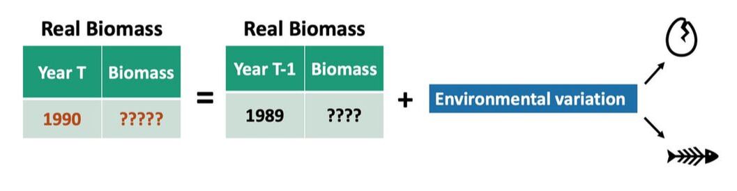
The random walk model is a category of model called a state-space model. State-space models have two conceptual levels - a hidden reality (in this case the true stock biomass at a given time) that we can’t directly measure or fully know, and the representation of reality (the stock biomass estimates we produce from the survey data) that we can measure and can use to approximate the hidden reality. In a random walk model, we assume that the (hidden) real stock biomass in a given year is a product of the real stock biomass the year before and some amount of uncertainty caused by environmental variability (such as births and deaths). An example is shown below.
The random walk model is a category of model called a state-space model. State-space models have two conceptual levels - a hidden reality (in this case the true stock biomass at a given time) that we can’t directly measure or fully know, and the representation of reality (the stock biomass estimates we produce from the survey data) that we can measure and can use to approximate the hidden reality. In a random walk model, we assume that the (hidden) real stock biomass in a given year is a product of the real stock biomass the year before and some amount of uncertainty caused by environmental variability (such as births and deaths). An example is shown below.
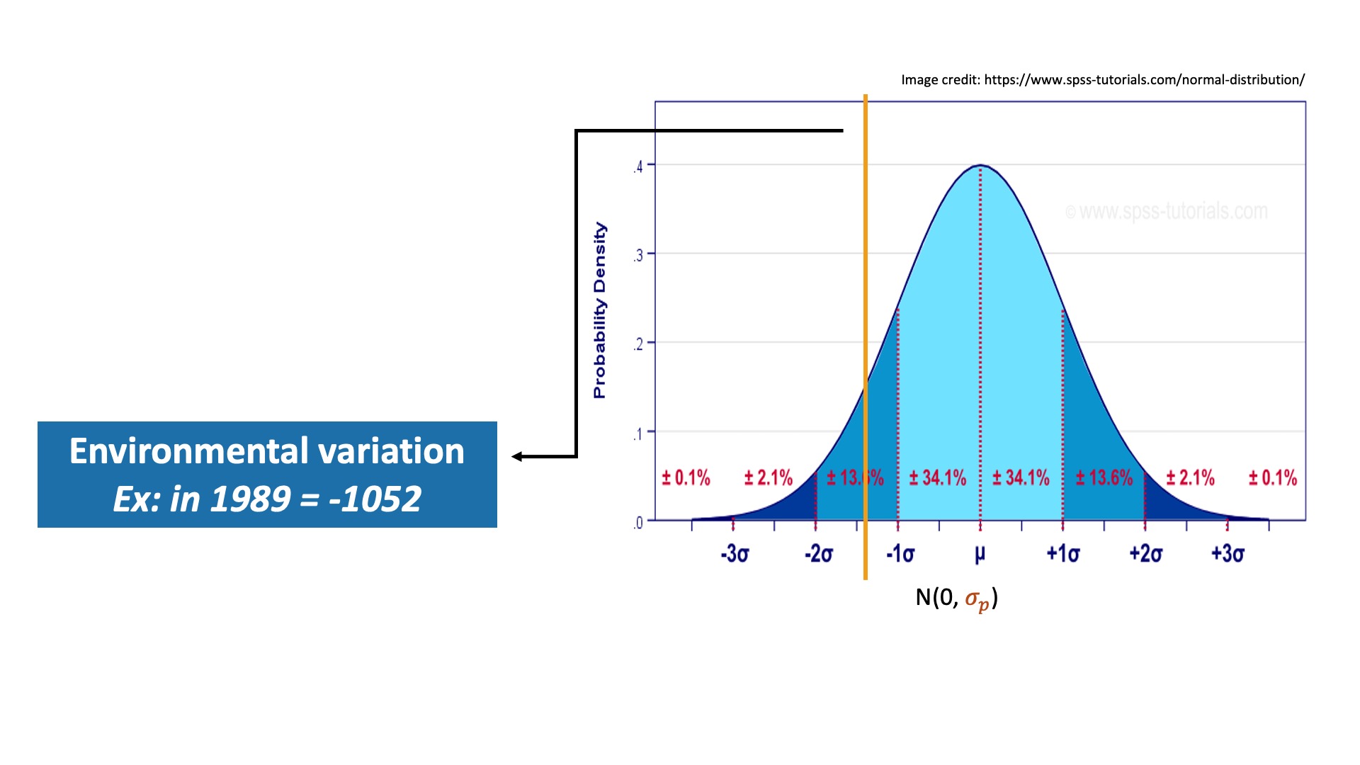
The actual value representing environmental variation in a given year is randomly drawn from a normal distribution, like the example pictured below. A normal distribution is characterized by an equal number of values on either side of the mean, with less likelihood of encountering values as the number of standard deviations from the mean increases. The percentages in the graphic indicate how many values are found within each section of the distribution. The mean of this normal distribution is set at 0, but the standard deviation (represented by σp in the graphic below, with the “p” standing for process error, another term for environmental variation), is estimated based on the survey data. This particular random walk model assumes that the distribution remains the same through time, meaning that we expect things like birth rates and death rates to be fairly consistent through time for these species.
Since there are two unknown values in the equation for hidden reality, we can’t determine this reality directly. To connect it to the survey data (which we do know), we assume that the survey data in a given year equals the real biomass in that year (which from the equation above we know is actually the biomass in the previous year plus environmental variation) combined with some amount of observation error, like in the example graphic below. Observation error refers to anything that affects our ability to accurately count the number of individuals in the observation area, and can arise from many sources. In the case of this data, some likely contributors include weather affecting the ability of the survey boats to go to every predetermined survey site, the fact that large portions of the bottom of the Gulf of Alaska are too rocky to trawl meaning they have to be left out of the survey, and human error, such as misidentifying fish when they are caught.
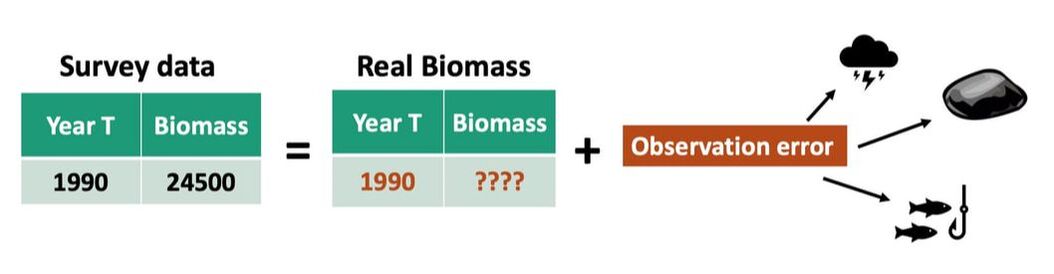
Similarly to environmental variation, the value to represent observation error in a given year is drawn from a normal distribution with a mean of zero and a standard deviation estimated from the data. Unlike environmental variation, we assume that the amount of observation error may change from year to year, based on individual conditions in each year, so a new distribution is calculated for each year (standard deviation is represented by σo,t below, where “o” stands for observation error and “t” stands for time, indicating it changes each year).

The random walk model doesn’t use spatial information as a variable, which means that an additional step is needed to estimate biomass separately for each subregion in the Gulf of Alaska. The survey data is separated out based on trawl location, and only the locations in a particular subregion are used to run the random walk model to produce estimates for that subregion. There are a couple of limitations with this method, primarily that the survey was not designed to randomly sample within subregions, so the assumption that the survey data will be random within a particular subregion in a particular year may not be a valid assumption. Additionally, there is no protocol ensuring that each subregion is sampled with the same intensity in the survey, meaning that some subregions may have more trawl sites (and therefore more data) than others in a given year or even through time. Scientists often have to work with assumptions that they know may be invalid while looking for alternate methods that don’t rely on those assumptions, and this particular issue is the impetus for this project.
Spatio-temporal model
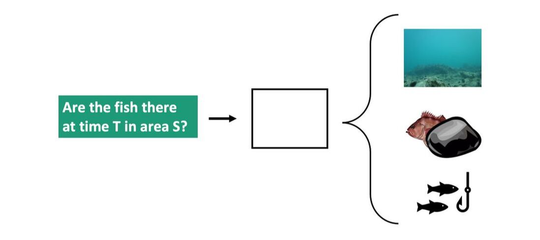
A spatio-temporal model, as implied by the name, refers to a model that uses both space and time as variables. The particular model used in this project is called a delta-General Linear Mixed Model (delta-GLMM). The logic of the model uses a two step process to predict stock biomass. The first step is to determine whether the fish are in a particular area at a particular time, and the answer is either yes, they are present, or no, they aren’t. If the fish aren’t present, the model does not try to explain why, although some reasons may include that they actually aren’t there, that they were there but the trawl didn’t capture them, or that they were there and they were captured but their species was misidentified through human error.
Spatio-temporal model
A spatio-temporal model, as implied by the name, refers to a model that uses both space and time as variables. The particular model used in this project is called a delta-General Linear Mixed Model (delta-GLMM). The logic of the model uses a two step process to predict stock biomass. The first step is to determine whether the fish are in a particular area at a particular time, and the answer is either yes, they are present, or no, they aren’t. If the fish aren’t present, the model does not try to explain why, although some reasons may include that they actually aren’t there, that they were there but the trawl didn’t capture them, or that they were there and they were captured but their species was misidentified through human error.
If the fish are present, then we can estimate biomass.
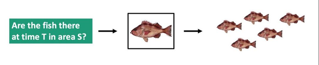
To model this logic, the delta-GLMM model uses two equations. One equation represents the probability that the fish are present in a particular area at a particular time (called encounter probability), and the other predicts the biomass. For this version of the model both equations use time, space and the interaction between time and space as variables.
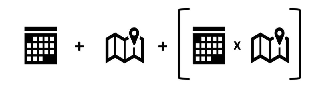
A strength of this type of model is that other variables can be added into either or both equations, so environmental factors like bottom type (rocky, sandy, etc.) and temperature could be included in future versions of the model.
To produce a predicted biomass at a particular area in a particular time, the encounter probability is multiplied by the estimated biomass. This means that if the encounter probability is small, the predicted biomass will be smaller. If the encounter probability is 0, then no biomass is predicted.
To produce a predicted biomass at a particular area in a particular time, the encounter probability is multiplied by the estimated biomass. This means that if the encounter probability is small, the predicted biomass will be smaller. If the encounter probability is 0, then no biomass is predicted.